CSN8010 Practical Lab 3 Vanilla CNN and Fine-Tune VGG16 - for Dogs and Cats Classification

Problem Framing

The aim of this lab is to predict the cat or dog class of an image using a Vanilla CNN and a Fine-Tune VGG16 model.

To compare the performance of both models, I will use the following metrics:

• Accuracy: The proportion of correct predictions made by the model.
• Precision: The proportion of true positive predictions made by the model out of all positive predictions.
• Recall: The proportion of true positive predictions made by the model out of all actual positive instances in the dataset.
• F1 Score: The harmonic mean of precision and recall, providing a balance between the two metrics.

import seaborn as sns
import matplotlib.pyplot as plt
from sklearn.metrics import confusion_matrix, classification_report, precision_recall_curve
import numpy as np
import os, pathlib
from imutils import paths
import random
from pathlib import Path
from PIL import Image
from collections import Counter
from tensorflow.keras.models import load_model
from tensorflow.keras import models, layers
from tensorflow.keras.applications import VGG16
from tensorflow.keras.callbacks import ModelCheckpoint, EarlyStopping

1. Get the data

The original dataset was downloaded from Kaggle, but this contained 25,000 thousand of photos. To create a smaller subset of the dataset, I executed the following Python script:

import os, shutil, pathlib

original_dir = pathlib.Path("../data/kaggle_dogs_vs_cats/train")
new_base_dir = pathlib.Path("../data/kaggle_dogs_vs_cats_small")

def make_subset(subset_name, start_index, end_index):
    for category in ("cat", "dog"):
        dir = new_base_dir / subset_name / category
        os.makedirs(dir)
        fnames = [f"{category}.{i}.jpg" for i in range(start_index, end_index)]
        for fname in fnames:
            shutil.copyfile(src=original_dir / fname,
                            dst=dir / fname)

make_subset("train", start_index=0, end_index=1000)
make_subset("validation", start_index=1000, end_index=1500)
make_subset("test", start_index=1500, end_index=2500)

Te new data set contains:

• 1000 training images.
• 500 validation images.
• 1000 test images per class

This reduces the dataset from 25,000 images to 5,000. Additionally, I split the dataset into three subsets train, validation, and test. The training set contains 1000 images per class, the validation set contains 500 images per class, and the test set contains 1000 images per class.

new_base_dir = pathlib.Path("./data/kaggle_dogs_vs_cats_small")

# Count the number of files in the new base directory
for subset in ["train", "validation", "test"]:
    num_files = len(list(paths.list_images(new_base_dir/subset)))
    print(f"Number of files in {subset}: {num_files}")

Number of files in train: 2000
Number of files in validation: 1000
Number of files in test: 2000

2. Data Exploration and Preprocessing

In this section, I will explore the dataset to understand its structure and content.

Show some random images from the dataset.

def show_random_images(base_path, subset, category, n=5):
    image_dir = Path(base_path) / subset / category
    images = list(image_dir.glob("*.jpg"))
    random_images = random.sample(images, n)

    plt.figure(figsize=(12, 5))
    for i, image_path in enumerate(random_images):
        img = Image.open(image_path)
        plt.subplot(1, n, i+1)
        plt.imshow(img)
        plt.axis("off")
        plt.title(image_path.name)
    plt.suptitle(f"Random {category} images from {subset} set", fontsize=12)
    plt.tight_layout()
    plt.show()

show_random_images(new_base_dir, 'train', 'cat')
show_random_images(new_base_dir, 'train', 'dog')

Validate the size of the images in the training set.

It is important to ensure that all images have the same size, as this is a requirement for training a CNN model. I will check the size of the images in the training set and print the frequency of each size.

sizes = []
modes = []

print(f"VALIDATING BALANCE OF DATASET...")

for subset in ["train", "validation", "test"]:
    print(f"\n--- {subset.upper()} ---")
    for category in ["cat", "dog"]:       
        count = len(list((new_base_dir / subset / category).glob("*.jpg")))
        print(f"{category}: {count}") 
        for path in (new_base_dir / subset / category).glob("*.jpg"):
            img = Image.open(path)
            sizes.append(img.size)
            modes.append(img.mode)  # 'RGB', 'L', 'RGBA', etc.
size_counts = Counter(sizes)
mode_counts = Counter(modes)

print(f"\nVALIDATING IMAGE SIZES (10 MOST COMMON)...")
for size, count in size_counts.most_common(10):
    print(f"{size}: {count} images")

print(f"\nVALIDATING IMAGE MODES...")
for mode, count in Counter(modes).most_common():
    print(f"{mode}: {count} images")

VALIDATING BALANCE OF DATASET...

--- TRAIN ---
cat: 1000
dog: 1000

--- VALIDATION ---
cat: 500
dog: 500

--- TEST ---
cat: 1000
dog: 1000

VALIDATING IMAGE SIZES (10 MOST COMMON)...
(499, 375): 578 images
(500, 374): 576 images
(375, 499): 59 images
(319, 240): 48 images
(374, 500): 47 images
(320, 239): 44 images
(499, 333): 41 images
(500, 332): 37 images
(500, 331): 25 images
(499, 332): 23 images

VALIDATING IMAGE MODES...
RGB: 5000 images

widths = [w for w, h in sizes]
heights = [h for w, h in sizes]

# Plot
plt.figure(figsize=(12, 5))

plt.subplot(1, 2, 1)
plt.hist(widths, bins=30, color='skyblue', edgecolor='black')
plt.title("Distribution of widths")
plt.xlabel("widths (pixels)")
plt.ylabel("Frequency")

plt.subplot(1, 2, 2)
plt.hist(heights, bins=30, color='salmon', edgecolor='black')
plt.title("Distribution of heights")
plt.xlabel("heights (pixels)")
plt.ylabel("Frequency")

plt.tight_layout()
plt.show()

In the exploration I found:

- There are some images with different sizes
- There are no images with different modes (all are RGB)
- Balance between classes (cats and dogs) is maintained in the training, validation, and test sets.

I will resize them to a common size of 150x150 pixels. This is a common practice in image classification tasks to ensure that all images have the same dimensions.

Preprocessing the images

In this section, I will preprocess the images to ensure they are in the correct format for training a CNN model. This includes resizing the images to a common size of 150x150 pixels, normalizing the pixel values to be between 0 and 1

# Mapping class name to numeric label
class_labels = {"cat": 0, "dog": 1}

def load_images_from_folder(folder_path, target_size=(150, 150)):

    x = []
    labels = []

    image_paths = list(paths.list_images(folder_path))
    random.shuffle(image_paths)


    for image_path, i in zip(image_paths, range(len(image_paths))):
        print(f"Loading image... {i} / {len(image_paths)}", end="\r")
        try:
            img = Image.open(image_path).resize(target_size) # Resize image to target size
            img = np.array(img).astype("float32") / 255.0  # Normalize to [0, 1]
            x.append(img)

            # Determine label from filename
            file_name = os.path.basename(image_path)
            if file_name.startswith("cat"):
                labels.append(class_labels["cat"])
            elif file_name.startswith("dog"):
                labels.append(class_labels["dog"])
            else:
                print(f"Warning: {file_name} does not match known class... Skipping...")

        except Exception as e:
            print(f"Error loading image {image_path}: {e}")

    x = np.array(x)
    labels = np.array(labels)

    print(f"✅ Loaded {len(x)} images from {folder_path.name}. Shape: {x.shape}")
    return x, labels

# Example usage:
x_train, y_train = load_images_from_folder(new_base_dir / "train", target_size=(150, 150))
x_val, y_val     = load_images_from_folder(new_base_dir / "validation", target_size=(150, 150))
x_test, y_test   = load_images_from_folder(new_base_dir / "test", target_size=(150, 150))

✅ Loaded 2000 images from train. Shape: (2000, 150, 150, 3)
✅ Loaded 1000 images from validation. Shape: (1000, 150, 150, 3)
✅ Loaded 2000 images from test. Shape: (2000, 150, 150, 3)

Showing the first image in the training set to verify that the preprocessing was successful.

This image is part of a 4D array with shape: (batch_size, height, width, channels).

When I access x_train[0], I am retrieving one image with shape (height, width, 3), represented as a 3D NumPy array. All data is normalized to the range [0, 1].

Showing one image and its label from the training set.

def show_image(x, label_batch, class_labels=class_labels, index=6):

    plt.figure(figsize=(6, 3))
    class_names = list(class_labels.keys())  # Get class
    idxs = np.random.choice(len(x), size=index, replace=False)

    for i, idx in enumerate(idxs):
        ax = plt.subplot(2, 3, i + 1)  # Arrange in 2*3 grid
        plt.imshow(x[idx])  
        plt.title(class_names[label_batch[idx]].title())  # Display the label
        plt.axis('off')  # Hide axis ticks
    plt.tight_layout()               
    plt.show()


show_image(x_train, y_train)

3. Architecture Design

In this section I will design the architecture of the CNN model.

CNN Sequential Model

Layers:

1. Conv2D
2. MaxPooling2D (32 filters, 3x3 kernel, ReLU activation)
3. Conv2D
4. MaxPooling2D (64 filters, 3x3 kernel, ReLU activation)
5. Flatten
6. Dense (hiddden neurons)
7. Dropout (0.5)
8. Final Dense with sigmoid (binary output)

model = models.Sequential() # Create a Sequential model, piled layer by layer

# FIRST LAYER: Conv2D (32) 
model.add(layers.Conv2D(
    filters=32,               # filter or feature detection size
    kernel_size=(3, 3),       # size of each filter (3x3 pixels)
    activation='relu',        # Relu activation Function to introduce non-linearity 
    input_shape=(150, 150, 3) # input shape: 150*150 pixels with 3 channels (RGB)
))

# SECOND LAYER: MaxPooling2D (reducing image size)
model.add(layers.MaxPooling2D(
    pool_size=(2, 2) # Only keep the maximum value in each 2x2 region
))

# THIRD LAYER: Conv2D (64) 
model.add(layers.Conv2D(
    filters=64,       # Increasing the number of filters to learn more complex features        
    kernel_size=(3, 3),       
    activation='relu',        
))

# FOURTH LAYER: MaxPooling2D (reducing image size)
model.add(layers.MaxPooling2D(
    pool_size=(2, 2) # Only keep the maximum value in each 2x2 region
))

# FIFTH LAYER: FLATTEN TO CONVERT 3D TO 1D
model.add(layers.Flatten()) # Output 1D to feed into Dense layers

# SIXTH LAYER: Dense (128) Fully Connected + Dropout (0.5)
model.add(layers.Dense(
    units=64,         # Number of neurons in this layer
    activation='relu' 
))

# SEVENTH LAYER: Dropout (0.6)
model.add(layers.Dropout(rate=0.6)) # Dropout to prevent overfitting

# FINAL LAYER: Dense (1) Output Layer
model.add(layers.Dense(
    units=1,            # Single neuron for binary output (0 or 1)
    activation='sigmoid' # Outputs a probability between 0 and 1
))

c:\Users\paula\github-classroom\CSCN8010 - Foundations ML Frameworks\CSCN8010-PR-Lab3\venvPR\Lib\site-packages\keras\src\layers\convolutional\base_conv.py:113: UserWarning: Do not pass an `input_shape`/`input_dim` argument to a layer. When using Sequential models, prefer using an `Input(shape)` object as the first layer in the model instead.
  super().__init__(activity_regularizer=activity_regularizer, **kwargs)

Summary

model.summary() 

Model: "sequential"

┏━━━━━━━━━━━━━━━━━━━━━━━━━━━━━━━━━┳━━━━━━━━━━━━━━━━━━━━━━━━┳━━━━━━━━━━━━━━━┓
┃ Layer (type)                    ┃ Output Shape           ┃       Param # ┃
┡━━━━━━━━━━━━━━━━━━━━━━━━━━━━━━━━━╇━━━━━━━━━━━━━━━━━━━━━━━━╇━━━━━━━━━━━━━━━┩
│ conv2d (Conv2D)                 │ (None, 148, 148, 32)   │           896 │
├─────────────────────────────────┼────────────────────────┼───────────────┤
│ max_pooling2d (MaxPooling2D)    │ (None, 74, 74, 32)     │             0 │
├─────────────────────────────────┼────────────────────────┼───────────────┤
│ conv2d_1 (Conv2D)               │ (None, 72, 72, 64)     │        18,496 │
├─────────────────────────────────┼────────────────────────┼───────────────┤
│ max_pooling2d_1 (MaxPooling2D)  │ (None, 36, 36, 64)     │             0 │
├─────────────────────────────────┼────────────────────────┼───────────────┤
│ flatten (Flatten)               │ (None, 82944)          │             0 │
├─────────────────────────────────┼────────────────────────┼───────────────┤
│ dense (Dense)                   │ (None, 64)             │     5,308,480 │
├─────────────────────────────────┼────────────────────────┼───────────────┤
│ dropout (Dropout)               │ (None, 64)             │             0 │
├─────────────────────────────────┼────────────────────────┼───────────────┤
│ dense_1 (Dense)                 │ (None, 1)              │            65 │
└─────────────────────────────────┴────────────────────────┴───────────────┘

 Total params: 5,327,937 (20.32 MB)

 Trainable params: 5,327,937 (20.32 MB)

 Non-trainable params: 0 (0.00 B)

# Compile the model with appropriate loss function and optimizer
model.compile(optimizer='adam', loss='binary_crossentropy', metrics=['accuracy'])

Setting the Callbacks and EarlyStopping

In this part of the lab, I set up callbacks to monitor the training process and save the best model based on validation accuracy.
I also used the EarlyStopping function to automatically stop the training when the model stopped improving, based on the patience parameter.
This helps prevent overfitting and ensures that the best-performing version of the model is retained.

# Create a callback to save the best version of the model (based on validation accuracy)
checkpoint_cb = ModelCheckpoint(
    filepath='best_model.h5',        # File where the best model will be saved
    monitor='val_accuracy',          # Metric to monitor
    save_best_only=True,             # Only save the model if it's the best so far
    mode='max',                      # We want to maximize validation accuracy
    verbose=1                        # Print a message each time the model is saved
)


earlystop_cb = EarlyStopping(
    monitor='val_accuracy',
    patience=3,              # Stop after 3 epochs without improvement
    restore_best_weights=True
)

Training the model

# Train the model using training data, validate on validation data
history = model.fit(
    x_train, y_train,               # Training data and labels
    epochs=20,                      # Number of times the model will see the full dataset
    batch_size=32,                 # Number of samples per gradient update
    validation_data=(x_val, y_val),# Validation data to evaluate on after each epoch
    callbacks=[checkpoint_cb, earlystop_cb]  # Save best model + stop if no improvement
)

Epoch 1/20
63/63 ━━━━━━━━━━━━━━━━━━━━ 0s 219ms/step - accuracy: 0.4858 - loss: 1.0680
Epoch 1: val_accuracy improved from None to 0.56200, saving model to best_model.h5

WARNING:absl:You are saving your model as an HDF5 file via `model.save()` or `keras.saving.save_model(model)`. This file format is considered legacy. We recommend using instead the native Keras format, e.g. `model.save('my_model.keras')` or `keras.saving.save_model(model, 'my_model.keras')`. 

63/63 ━━━━━━━━━━━━━━━━━━━━ 17s 258ms/step - accuracy: 0.5185 - loss: 0.8091 - val_accuracy: 0.5620 - val_loss: 0.6880
Epoch 2/20
63/63 ━━━━━━━━━━━━━━━━━━━━ 0s 215ms/step - accuracy: 0.5892 - loss: 0.6764
Epoch 2: val_accuracy improved from 0.56200 to 0.59300, saving model to best_model.h5

WARNING:absl:You are saving your model as an HDF5 file via `model.save()` or `keras.saving.save_model(model)`. This file format is considered legacy. We recommend using instead the native Keras format, e.g. `model.save('my_model.keras')` or `keras.saving.save_model(model, 'my_model.keras')`. 

63/63 ━━━━━━━━━━━━━━━━━━━━ 15s 241ms/step - accuracy: 0.5920 - loss: 0.6707 - val_accuracy: 0.5930 - val_loss: 0.6616
Epoch 3/20
63/63 ━━━━━━━━━━━━━━━━━━━━ 0s 203ms/step - accuracy: 0.6223 - loss: 0.6605
Epoch 3: val_accuracy improved from 0.59300 to 0.63600, saving model to best_model.h5

WARNING:absl:You are saving your model as an HDF5 file via `model.save()` or `keras.saving.save_model(model)`. This file format is considered legacy. We recommend using instead the native Keras format, e.g. `model.save('my_model.keras')` or `keras.saving.save_model(model, 'my_model.keras')`. 

63/63 ━━━━━━━━━━━━━━━━━━━━ 14s 230ms/step - accuracy: 0.6215 - loss: 0.6591 - val_accuracy: 0.6360 - val_loss: 0.6568
Epoch 4/20
63/63 ━━━━━━━━━━━━━━━━━━━━ 0s 202ms/step - accuracy: 0.6748 - loss: 0.6077
Epoch 4: val_accuracy improved from 0.63600 to 0.65900, saving model to best_model.h5

WARNING:absl:You are saving your model as an HDF5 file via `model.save()` or `keras.saving.save_model(model)`. This file format is considered legacy. We recommend using instead the native Keras format, e.g. `model.save('my_model.keras')` or `keras.saving.save_model(model, 'my_model.keras')`. 

63/63 ━━━━━━━━━━━━━━━━━━━━ 14s 228ms/step - accuracy: 0.6900 - loss: 0.5955 - val_accuracy: 0.6590 - val_loss: 0.6394
Epoch 5/20
63/63 ━━━━━━━━━━━━━━━━━━━━ 0s 208ms/step - accuracy: 0.7484 - loss: 0.5283
Epoch 5: val_accuracy improved from 0.65900 to 0.66800, saving model to best_model.h5

WARNING:absl:You are saving your model as an HDF5 file via `model.save()` or `keras.saving.save_model(model)`. This file format is considered legacy. We recommend using instead the native Keras format, e.g. `model.save('my_model.keras')` or `keras.saving.save_model(model, 'my_model.keras')`. 

63/63 ━━━━━━━━━━━━━━━━━━━━ 15s 235ms/step - accuracy: 0.7435 - loss: 0.5307 - val_accuracy: 0.6680 - val_loss: 0.6374
Epoch 6/20
Epoch 6/20
63/63 ━━━━━━━━━━━━━━━━━━━━ 0s 206ms/step - accuracy: 0.7911 - loss: 0.4498
Epoch 6: val_accuracy did not improve from 0.66800
63/63 ━━━━━━━━━━━━━━━━━━━━ 14s 229ms/step - accuracy: 0.7825 - loss: 0.4572 - val_accuracy: 0.6360 - val_loss: 0.6985
Epoch 7/20
63/63 ━━━━━━━━━━━━━━━━━━━━ 0s 199ms/step - accuracy: 0.8571 - loss: 0.3561
Epoch 7: val_accuracy did not improve from 0.66800
63/63 ━━━━━━━━━━━━━━━━━━━━ 14s 222ms/step - accuracy: 0.8445 - loss: 0.3658 - val_accuracy: 0.6560 - val_loss: 0.7023
Epoch 8/20
63/63 ━━━━━━━━━━━━━━━━━━━━ 0s 196ms/step - accuracy: 0.8635 - loss: 0.3269
Epoch 8: val_accuracy did not improve from 0.66800
63/63 ━━━━━━━━━━━━━━━━━━━━ 14s 220ms/step - accuracy: 0.8745 - loss: 0.3025 - val_accuracy: 0.6590 - val_loss: 0.7930

# Accuracy plot
plt.figure(figsize=(8, 5))

plt.subplot(1, 2, 1)
plt.plot(history.history['accuracy'], label='Train Accuracy')
plt.plot(history.history['val_accuracy'], label='Validation Accuracy')
plt.title('Accuracy over epochs')
plt.xlabel('Epoch')
plt.ylabel('Accuracy')
plt.legend()

# Loss plot
plt.subplot(1, 2, 2)
plt.plot(history.history['loss'], label='Train Loss')
plt.plot(history.history['val_loss'], label='Validation Loss')
plt.title('Loss over epochs')
plt.xlabel('Epoch')
plt.ylabel('Loss')
plt.legend()

plt.tight_layout()
plt.show()

• The accuracy graph shows that the training accuracy increases while the validation accuracy decreases, indicating overfitting.
• In the loss graph, we can see that the training loss decreases while the validation loss increases, which is also a sign of overfitting.

Those graphs will show the training and validation accuracy and loss over the epochs.

The Custom CNN model completed its training in 8 epochs, as determined by the EarlyStopping callback based on validation accuracy. This indicates that the model reached its best performance before the maximum number of epochs was reached.

Fine- Tune VGG16

In this step, I will use a pre-trained VGG16 model as a base and fine-tune it for the dog vs cat classification task. The VGG16 model is a well-known convolutional neural network architecture that has been pre-trained on the ImageNet dataset.

Then, I going to add my own layers on the top of the VGG16 model to adapt it to the dog vs cat classification task.

# Load the VGG16 base model without the top classifier layers
vgg_base = VGG16(
    weights='imagenet',        # Load pre-trained weights
    include_top=False,         
    input_shape=(150, 150, 3)  # Match the shape of your input images
)

To do not change the weights of the VGG16 model, I will freeze the layers of the base model. This means that the weights of the VGG16 model will not be updated during training.

vgg_base.trainable = False  # Freeze all convolutional layers

Creating my top layers

1. Flatten
2. Dense (hidden neurons)
3. Dropout (0.5)
4. Final Dense with sigmoid (binary output)

# Create a new model on top of the frozen VGG16 base
model_vgg = models.Sequential()

# Add the VGG16 convolutional base
model_vgg.add(vgg_base)

# Add custom classifier on top

# FIRST LAYER: Flatten the output of the conv base
model_vgg.add(layers.Flatten())            

# SECOND LAYER: Fully connected layer
model_vgg.add(layers.Dense(64, activation='relu'))     

# THIRD LAYER: Dropout for regularization
model_vgg.add(layers.Dropout(0.5))  

#FOURTH LAYER: Final Dense layer for binary classification (Output layer)
model_vgg.add(layers.Dense(1, activation='sigmoid'))    

# Compile the model with appropriate loss function and optimizer
model_vgg.compile(optimizer='adam', loss='binary_crossentropy', metrics=['accuracy'])

Setting the callbacks and earlystop for VGG16

# Define callbacks
checkpoint_cb = ModelCheckpoint(
    filepath='best_vgg_model.h5',     # File to save best version of VGG16 model
    monitor='val_accuracy',           # Watch validation accuracy
    save_best_only=True,              # Save only the best model
    mode='max',
    verbose=1
)


earlystop_cb = EarlyStopping(
    monitor='val_accuracy',          # Stop if val accuracy stops improving
    patience=3,                      # Wait 3 epochs before stopping
    restore_best_weights=True
)

Training the model with VGG16

# Train the model using training data, validate on validation data
history_vgg = model_vgg.fit(
    x_train, y_train,
    epochs=20,
    batch_size=32,
    validation_data=(x_val, y_val),
    callbacks=[checkpoint_cb, earlystop_cb]
)

Epoch 1/20
63/63 ━━━━━━━━━━━━━━━━━━━━ 0s 812ms/step - accuracy: 0.6986 - loss: 0.6018
Epoch 1: val_accuracy improved from None to 0.86200, saving model to best_vgg_model.h5

WARNING:absl:You are saving your model as an HDF5 file via `model.save()` or `keras.saving.save_model(model)`. This file format is considered legacy. We recommend using instead the native Keras format, e.g. `model.save('my_model.keras')` or `keras.saving.save_model(model, 'my_model.keras')`. 

63/63 ━━━━━━━━━━━━━━━━━━━━ 81s 1s/step - accuracy: 0.7950 - loss: 0.4427 - val_accuracy: 0.8620 - val_loss: 0.2879
Epoch 2/20
63/63 ━━━━━━━━━━━━━━━━━━━━ 0s 853ms/step - accuracy: 0.8860 - loss: 0.2894
Epoch 2: val_accuracy improved from 0.86200 to 0.89500, saving model to best_vgg_model.h5

WARNING:absl:You are saving your model as an HDF5 file via `model.save()` or `keras.saving.save_model(model)`. This file format is considered legacy. We recommend using instead the native Keras format, e.g. `model.save('my_model.keras')` or `keras.saving.save_model(model, 'my_model.keras')`. 

63/63 ━━━━━━━━━━━━━━━━━━━━ 80s 1s/step - accuracy: 0.8825 - loss: 0.2798 - val_accuracy: 0.8950 - val_loss: 0.2659
Epoch 3/20
63/63 ━━━━━━━━━━━━━━━━━━━━ 0s 836ms/step - accuracy: 0.9142 - loss: 0.2128
Epoch 3: val_accuracy improved from 0.89500 to 0.90200, saving model to best_vgg_model.h5

WARNING:absl:You are saving your model as an HDF5 file via `model.save()` or `keras.saving.save_model(model)`. This file format is considered legacy. We recommend using instead the native Keras format, e.g. `model.save('my_model.keras')` or `keras.saving.save_model(model, 'my_model.keras')`. 

63/63 ━━━━━━━━━━━━━━━━━━━━ 79s 1s/step - accuracy: 0.9100 - loss: 0.2298 - val_accuracy: 0.9020 - val_loss: 0.2342
Epoch 4/20
63/63 ━━━━━━━━━━━━━━━━━━━━ 0s 818ms/step - accuracy: 0.9249 - loss: 0.2011
Epoch 4: val_accuracy did not improve from 0.90200
63/63 ━━━━━━━━━━━━━━━━━━━━ 77s 1s/step - accuracy: 0.9180 - loss: 0.2068 - val_accuracy: 0.8980 - val_loss: 0.2361
Epoch 5/20
63/63 ━━━━━━━━━━━━━━━━━━━━ 0s 830ms/step - accuracy: 0.9255 - loss: 0.1737
Epoch 5: val_accuracy improved from 0.90200 to 0.90300, saving model to best_vgg_model.h5

WARNING:absl:You are saving your model as an HDF5 file via `model.save()` or `keras.saving.save_model(model)`. This file format is considered legacy. We recommend using instead the native Keras format, e.g. `model.save('my_model.keras')` or `keras.saving.save_model(model, 'my_model.keras')`. 

63/63 ━━━━━━━━━━━━━━━━━━━━ 78s 1s/step - accuracy: 0.9355 - loss: 0.1576 - val_accuracy: 0.9030 - val_loss: 0.2320
Epoch 6/20
63/63 ━━━━━━━━━━━━━━━━━━━━ 0s 881ms/step - accuracy: 0.9474 - loss: 0.1402
Epoch 6: val_accuracy did not improve from 0.90300
63/63 ━━━━━━━━━━━━━━━━━━━━ 82s 1s/step - accuracy: 0.9475 - loss: 0.1414 - val_accuracy: 0.8960 - val_loss: 0.2591
Epoch 7/20
63/63 ━━━━━━━━━━━━━━━━━━━━ 0s 843ms/step - accuracy: 0.9588 - loss: 0.1036
Epoch 7: val_accuracy improved from 0.90300 to 0.90700, saving model to best_vgg_model.h5

WARNING:absl:You are saving your model as an HDF5 file via `model.save()` or `keras.saving.save_model(model)`. This file format is considered legacy. We recommend using instead the native Keras format, e.g. `model.save('my_model.keras')` or `keras.saving.save_model(model, 'my_model.keras')`. 

63/63 ━━━━━━━━━━━━━━━━━━━━ 80s 1s/step - accuracy: 0.9530 - loss: 0.1115 - val_accuracy: 0.9070 - val_loss: 0.2334
Epoch 8/20
63/63 ━━━━━━━━━━━━━━━━━━━━ 0s 830ms/step - accuracy: 0.9600 - loss: 0.1047
Epoch 8: val_accuracy did not improve from 0.90700
63/63 ━━━━━━━━━━━━━━━━━━━━ 78s 1s/step - accuracy: 0.9620 - loss: 0.1008 - val_accuracy: 0.9070 - val_loss: 0.2454
Epoch 9/20
63/63 ━━━━━━━━━━━━━━━━━━━━ 0s 811ms/step - accuracy: 0.9662 - loss: 0.0795
Epoch 9: val_accuracy improved from 0.90700 to 0.90800, saving model to best_vgg_model.h5

WARNING:absl:You are saving your model as an HDF5 file via `model.save()` or `keras.saving.save_model(model)`. This file format is considered legacy. We recommend using instead the native Keras format, e.g. `model.save('my_model.keras')` or `keras.saving.save_model(model, 'my_model.keras')`. 

63/63 ━━━━━━━━━━━━━━━━━━━━ 77s 1s/step - accuracy: 0.9645 - loss: 0.0871 - val_accuracy: 0.9080 - val_loss: 0.2428
Epoch 10/20
63/63 ━━━━━━━━━━━━━━━━━━━━ 0s 834ms/step - accuracy: 0.9700 - loss: 0.0721
Epoch 10: val_accuracy did not improve from 0.90800
63/63 ━━━━━━━━━━━━━━━━━━━━ 78s 1s/step - accuracy: 0.9745 - loss: 0.0678 - val_accuracy: 0.9030 - val_loss: 0.2726
Epoch 11/20
63/63 ━━━━━━━━━━━━━━━━━━━━ 0s 803ms/step - accuracy: 0.9784 - loss: 0.0629
Epoch 11: val_accuracy did not improve from 0.90800
63/63 ━━━━━━━━━━━━━━━━━━━━ 75s 1s/step - accuracy: 0.9815 - loss: 0.0603 - val_accuracy: 0.9060 - val_loss: 0.2581
Epoch 12/20
63/63 ━━━━━━━━━━━━━━━━━━━━ 0s 813ms/step - accuracy: 0.9908 - loss: 0.0411
Epoch 12: val_accuracy improved from 0.90800 to 0.91500, saving model to best_vgg_model.h5

WARNING:absl:You are saving your model as an HDF5 file via `model.save()` or `keras.saving.save_model(model)`. This file format is considered legacy. We recommend using instead the native Keras format, e.g. `model.save('my_model.keras')` or `keras.saving.save_model(model, 'my_model.keras')`. 

63/63 ━━━━━━━━━━━━━━━━━━━━ 77s 1s/step - accuracy: 0.9865 - loss: 0.0448 - val_accuracy: 0.9150 - val_loss: 0.2626
Epoch 13/20
Epoch 13/20
63/63 ━━━━━━━━━━━━━━━━━━━━ 0s 783ms/step - accuracy: 0.9857 - loss: 0.0472
Epoch 13: val_accuracy did not improve from 0.91500
63/63 ━━━━━━━━━━━━━━━━━━━━ 75s 1s/step - accuracy: 0.9865 - loss: 0.0462 - val_accuracy: 0.9070 - val_loss: 0.2761
Epoch 14/20
63/63 ━━━━━━━━━━━━━━━━━━━━ 0s 817ms/step - accuracy: 0.9910 - loss: 0.0362
Epoch 14: val_accuracy did not improve from 0.91500
63/63 ━━━━━━━━━━━━━━━━━━━━ 79s 1s/step - accuracy: 0.9875 - loss: 0.0408 - val_accuracy: 0.8990 - val_loss: 0.3166
Epoch 15/20
63/63 ━━━━━━━━━━━━━━━━━━━━ 0s 813ms/step - accuracy: 0.9837 - loss: 0.0451
Epoch 15: val_accuracy did not improve from 0.91500
63/63 ━━━━━━━━━━━━━━━━━━━━ 78s 1s/step - accuracy: 0.9865 - loss: 0.0422 - val_accuracy: 0.9090 - val_loss: 0.2819

# Accuracy plot
plt.figure(figsize=(8, 5))

plt.subplot(1, 2, 1)
plt.plot(history_vgg.history['accuracy'], label='Train Accuracy')
plt.plot(history_vgg.history['val_accuracy'], label='Validation Accuracy')
plt.title('Accuracy over epochs')
plt.xlabel('Epoch')
plt.ylabel('Accuracy')
plt.legend()

# Loss plot
plt.subplot(1, 2, 2)
plt.plot(history_vgg.history['loss'], label='Train Loss')
plt.plot(history_vgg.history['val_loss'], label='Validation Loss')
plt.title('Loss over epochs')
plt.xlabel('Epoch')
plt.ylabel('Loss')
plt.legend()

plt.tight_layout()
plt.show()

The accuracy graph shows that while training accuracy steadily increases, validation accuracy begins to fluctuate after a few epochs. The EarlyStopping function effectively halted training to prevent overfitting.

The VGG16 model completed its training in 15 epochs. This indicates that the model reached its best performance before the maximum number of epochs was reached

4. Performing the models

Loading the best version of each model. To automate this, I going to create a function and then evaluate both conventional and using VGG.

Creating a function to evaluate models

def evaluate_models(name, model_path):
    best_model = load_model(model_path)
    # Predictions
    y_probs = best_model.predict(x_test)
    y_preds = (y_probs > 0.5).astype("int32") # Convert probs to class
    
    # Accuracy and loss
    test_loss, test_accuracy = best_model.evaluate(x_test, y_test)
    print(f"\n🔍 Evaluation for {name}")
    print(f"Test Accuracy: {test_accuracy:.4f}")
    print(f"Test Loss: {test_loss:.4f}")

    # Confusion Matrix - Positives and False
    cm = confusion_matrix(y_test, y_preds)
    plt.figure(figsize=(5,4))
    sns.heatmap(cm, annot=True, fmt='d', cmap='Blues')
    plt.title(f"Confusion Matrix – {name}")
    plt.xlabel("Predicted")
    plt.ylabel("Actual")
    plt.show()

    #classification_report - precision, recall y F1-score
    print("Classification Report:")
    print(classification_report(y_test, y_preds, target_names=["Cat", "Dog"]))


    # precision_recall_curve- Variation
    precisions, recalls, thresholds = precision_recall_curve(y_test, y_probs)
    
    plt.figure(figsize=(6,5))
    plt.plot(recalls, precisions, marker='.')
    plt.title(f"Precision–Recall Curve – {name}")
    plt.xlabel("Recall")
    plt.ylabel("Precision")
    plt.grid(True)
    plt.show()

Test Set Evaluation – Custom Convolutional Model

evaluate_models('Custom CNN','best_model.h5')

WARNING:absl:Compiled the loaded model, but the compiled metrics have yet to be built. `model.compile_metrics` will be empty until you train or evaluate the model.

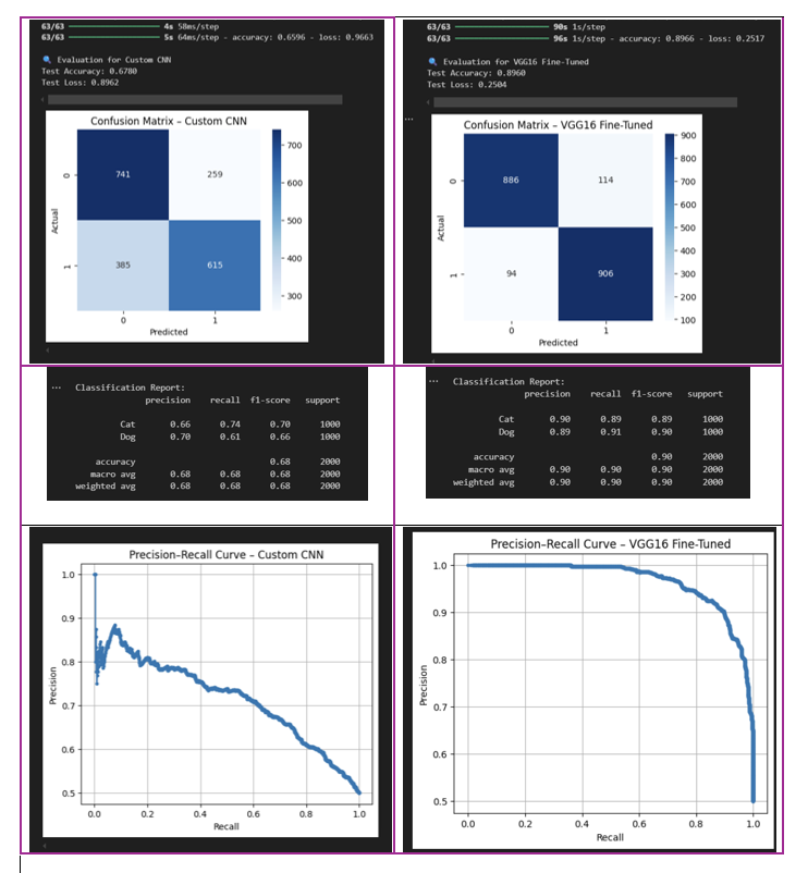
63/63 ━━━━━━━━━━━━━━━━━━━━ 3s 48ms/step
63/63 ━━━━━━━━━━━━━━━━━━━━ 3s 47ms/step - accuracy: 0.6785 - loss: 1.0055

🔍 Evaluation for Custom CNN
Test Accuracy: 0.6785
Test Loss: 1.0055

Classification Report:
              precision    recall  f1-score   support

         Cat       0.69      0.65      0.67      1000
         Dog       0.67      0.70      0.69      1000

    accuracy                           0.68      2000
   macro avg       0.68      0.68      0.68      2000
weighted avg       0.68      0.68      0.68      2000

The accuracy in the test set is 0.67, which indicates that the model is not performing well on unseen data. This is likely due to overfitting, as the model performs well on the training and validation sets but fails to generalize to new data.

Test Set Evaluation – VGG16 Fine-Tuned Model

evaluate_models("VGG16 Fine-Tuned", "best_vgg_model.h5")

WARNING:absl:Compiled the loaded model, but the compiled metrics have yet to be built. `model.compile_metrics` will be empty until you train or evaluate the model.

63/63 ━━━━━━━━━━━━━━━━━━━━ 51s 799ms/step
63/63 ━━━━━━━━━━━━━━━━━━━━ 52s 814ms/step - accuracy: 0.8930 - loss: 0.2997

🔍 Evaluation for VGG16 Fine-Tuned
Test Accuracy: 0.8930
Test Loss: 0.2997

Classification Report:
              precision    recall  f1-score   support

         Cat       0.89      0.89      0.89      1000
         Dog       0.89      0.89      0.89      1000

    accuracy                           0.89      2000
   macro avg       0.89      0.89      0.89      2000
weighted avg       0.89      0.89      0.89      2000

The accuracy with VGG16 reached 0.89, which shows a clear improvement compared to the previous model's accuracy of 0.67. Its validation performance was more stable, and the use of EarlyStopping helped avoid overfitting. Overall, the model generalizes well and is expected to perform effectively on new, unseen data

Conclusions - Comparing models

The VGG16 Fine-Tuned maintained high precision even at high levels of recall. In contrast, the custom CNN model showed an imbalance between precision and recall. The F1 Score was significantly better for the VGG16 Fine-Tuned, reaching 89% for dogs and 90% for cats. A visual summary of this comparison is provided in the next image:

Showing Misclassified Images

To show some examples from the test set that were misclassified for each model. I going to create a function too.

def show_misclassified_images(model_path, name, num_images=9):
    model = load_model(model_path)
    y_probs = model.predict(x_test)
    y_preds = (y_probs > 0.5).astype("int32")

    misclassified_idxs = np.where(y_preds.flatten() != y_test)[0]

    if len(misclassified_idxs) == 0:
        print(f"No misclassified images found for {name}.")
        return

    sample_idxs = np.random.choice(misclassified_idxs, size=min(num_images, len(misclassified_idxs)), replace=False)

    plt.figure(figsize=(12, 6))
    for i, idx in enumerate(sample_idxs):
        plt.subplot(3, 3, i + 1)
        plt.imshow(x_test[idx])
        true_label = "Dog" if y_test[idx] == 1 else "Cat"
        pred_label = "Dog" if y_preds[idx] == 1 else "Cat"
        plt.title(f"True: {true_label}, Pred: {pred_label}")
        plt.axis('off')

    plt.suptitle(f"Misclassified Examples – {name}", fontsize=14)
    plt.tight_layout()
    plt.show()

The images below show the true label vs. the predicted label for each failure case.

show_misclassified_images("best_model.h5", "Custom CNN")

WARNING:absl:Compiled the loaded model, but the compiled metrics have yet to be built. `model.compile_metrics` will be empty until you train or evaluate the model.

63/63 ━━━━━━━━━━━━━━━━━━━━ 3s 49ms/step

The Custom CNN model reveals specific types of images where it tends to struggle:

• Images containing more than one pet
• Black and white dogs, which are sometimes confused with cats
• Blurry backgrounds that make the subject harder to identify
• Unusual angles or rotations, as well as non-standard backgrounds

show_misclassified_images("best_vgg_model.h5", "VGG16 Fine-Tuned")

WARNING:absl:Compiled the loaded model, but the compiled metrics have yet to be built. `model.compile_metrics` will be empty until you train or evaluate the model.

63/63 ━━━━━━━━━━━━━━━━━━━━ 50s 786ms/step

The VGG16 Fine-Tuned model misclassified some:

• dogs with unusual poses and faces
• As well as small pets or pets with objects partially covering their picture (e.g., toys, blankets, or hands).
• Pictures with letters.

These situations may obscure key visual features used by the model to differentiate classes.

5. Final Conclusions

As demonstrated in the previous sections, and after comparing both models, the VGG16 Fine-Tuned model clearly outperformed the custom CNN across all key evaluation metrics: accuracy, precision, recall, F1-score, and overall stability on the test set.

In addition, it made fewer classification errors, as shown in the confusion matrix and visual analysis of misclassified examples.

Although the VGG16-based model takes more than 15 minutes to train, the improvement in accuracy and generalization makes the trade-off worthwhile.

Therefore, the VGG16 Fine-Tuned model is more suitable for this binary image classification task.